COVID 19 Analysis(India)

Radhesh Started Speaking:

Hello! Everyone I am hoping that you all will be fine .

This is the new blog about an analysis of Covid19 in india So, lets get started

Downloading the dataset:

i downloaded the dataset from:

https://www.kaggle.com/sudalairajkumar/covid19-in-india

Importing necessory libraries:-

import numpy as np
import pandas as pd
import matplotlib.pyplot as plt
import seaborn as sns
sns.set()
import warnings
warnings.filterwarnings('ignore')

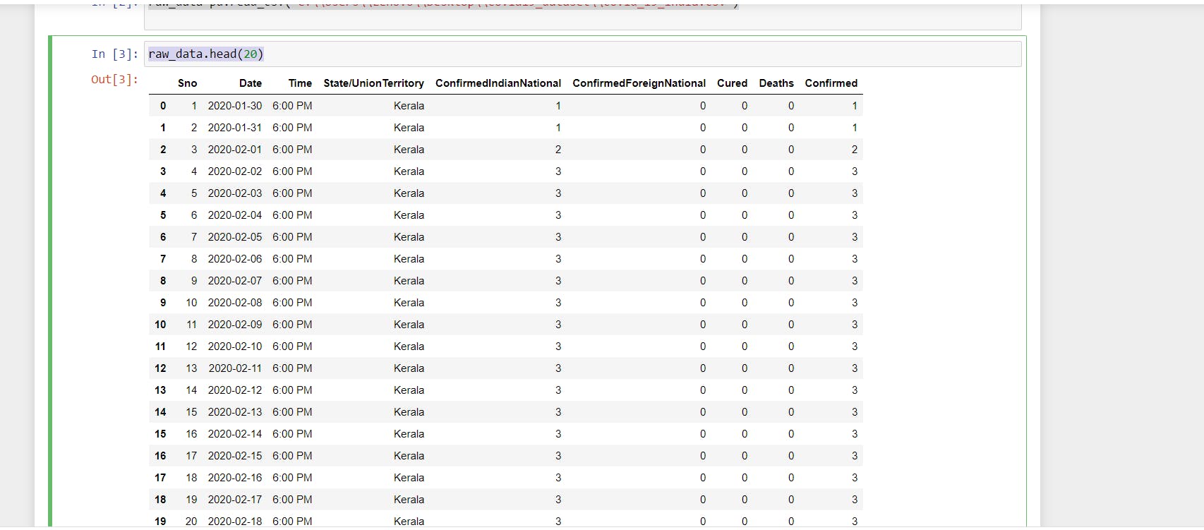
After downloading the dataset i opened the dataset into my jupyter notebook,
Then analyzed the dataset like what are and how many features are in there or what is the trait of the data.

raw_data=pd.read_csv('C:\\Users\\Lenovo\\Desktop\\covid19_dataset\\covid_19_india.csv')
raw_data.head(20)

Output:

Screenshot (28).png

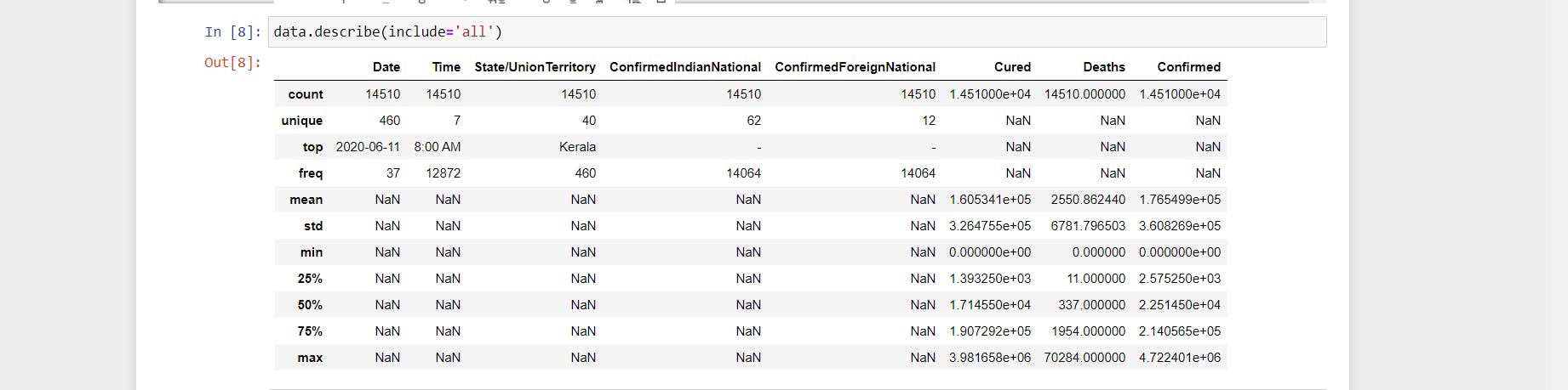
Now, checking the traits:

data=raw_data.copy()
data.describe(include='all')

Output:

Screenshot (29).png

Now,checking the relationship between deaths , cure and confirm cases in states:

For confirm:-

dataset=data.groupby('State/UnionTerritory').Confirmed.sum().sort_values(ascending=False).head(60)
plt.figure(figsize=(6,10))
sns.set_style('whitegrid')
ax=sns.scatterplot(dataset.values,dataset.index)
plt.suptitle('Graph b/w States and Confirmed cases')
ax.set_xlabel('Confirm cases');

Output:

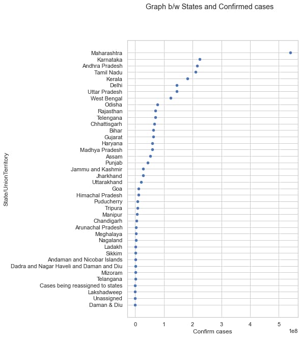
Conclusion: Maharastra has highest no. of positive cases

Let's analyze which state has highest no. of Death Rate:-

dataset1=data.groupby('State/UnionTerritory').Deaths.sum().sort_values(ascending=False).head(60)
plt.figure(figsize=(6,10))
sns.set_style('darkgrid')
ax=sns.barplot(dataset1.values,dataset1.index)
ax.set_xlabel("Deaths(in percent)")


sns.set_style('whitegrid')

plt.suptitle('Graph b/w States and Deaths',);

Output:

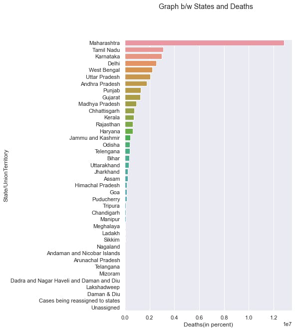
from above graph it is clear that Maharastra has highest no. of death rates

Now, for Recovery Rate:-

dataset2=data.groupby('State/UnionTerritory').Cured.sum().sort_values(ascending=False).head(70)
plt.figure(figsize=(6,10))
sns.set_style('darkgrid')
ax=sns.lineplot(dataset2.values,dataset2.index)
plt.suptitle('Graph b/w States and Cured cases')
ax.set_xlabel('Cured(in percent)');

Output:

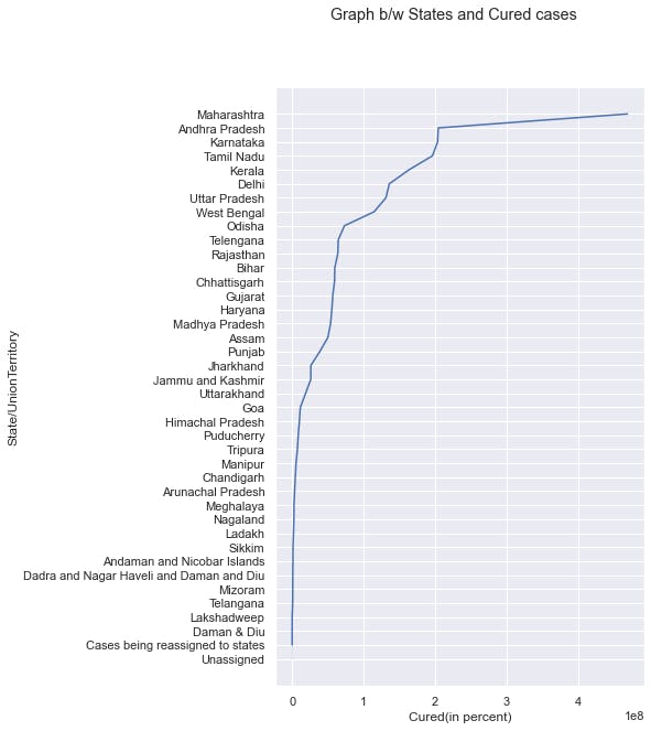
From above graphical analysis we can conclude that the Top Five state in Death ,Confirm,Cure Cases are:

Maharastra

Andhra Pradesh

Karnatka

Delhi

West Bengal

Now, checking the Rate of Deaths V/S Rates of Recovery:-

plt.figure(figsize=(11,10))
plt.suptitle("Graph B/W Death Rate and Recovery Rate in india")

sns.lineplot(
    data=data[['Cured','Deaths']]
    ,markers=False, dashes=True,palette='muted',err_style='bars',ci=None
)
sns.set_style("whitegrid")

plt.show()

r vs D.png

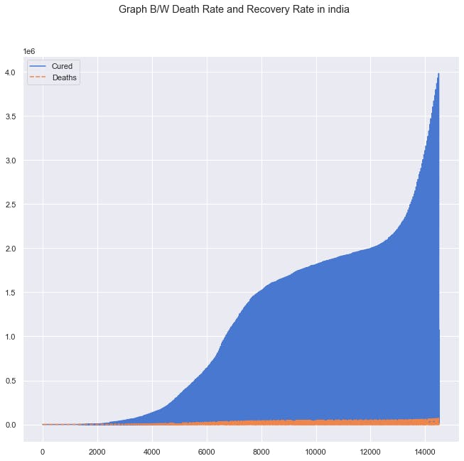
Means Recovery Rate is Higher Than The Death Rate In India Which Is a Good Sign:)

Now, Checking the vaccination:-

raw_vaccination=pd.read_csv('C:\\Users\\Lenovo\\Desktop\\covid19_dataset\\covid_vaccine_statewise.csv')
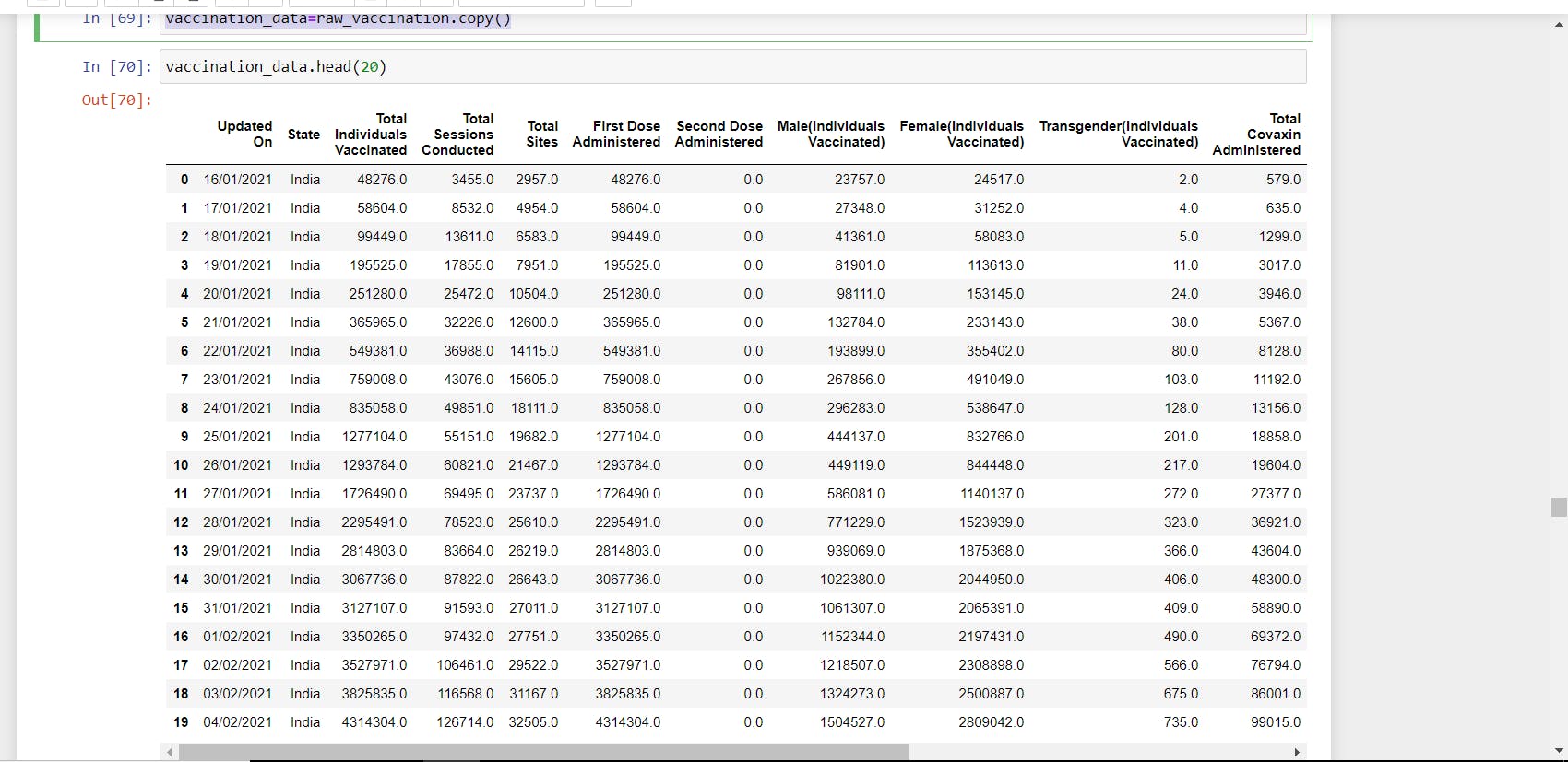
vaccination_data=raw_vaccination.copy()
vaccination_data.head(20)

Output:

Screenshot (30).png

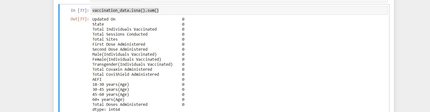
Checking for Null Values:

vaccination_data.isna().sum()

Output:

Screenshot (31).png

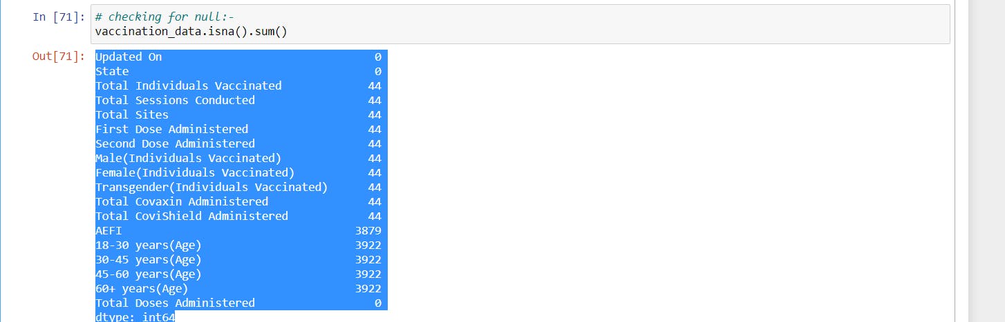
So there are null values present in our dataset

Fill the null values according to median

To fill this i created a function:

def filling_Data(col):
  if vaccination_data[col].isna().sum()==0:
      pass
  else:
      vaccination_data[col]=vaccination_data[col].fillna(vaccination_data[col].median())
  return vaccination_data[col]

Now, pass the values to the function:

for col in vaccination_data.columns:
    filling_Data(col)

Now again check the null values:-

vaccination_data.isna().sum()

Output:

Screenshot (32).png

Now,checking relationship between total individuas vaccinated and session:-

plt.figure(figsize=(9,8))
sns.set_style('whitegrid', rc={"lines.linewidth": 0.7})
sns.lineplot(vaccination_data['State'],vaccination_data['Total Sessions Conducted'])
sns.lineplot(vaccination_data['State'],vaccination_data['Total Individuals Vaccinated'])
plt.tight_layout()
plt.xticks(rotation=90)
plt.legend(['Total_sessions','total_individuals vaccinated'])
plt.show()

Output:-

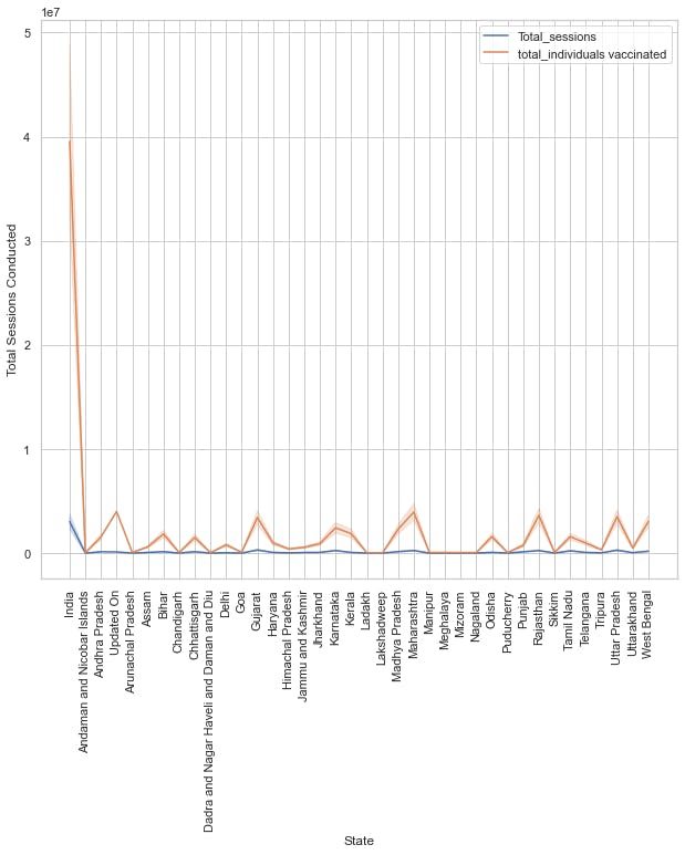
Above graph reflects that vaccination rate is higher in india

Now, checking the Difference B/W first dose and second dose:-

plt.figure(figsize=(9,8))
sns.set_style('whitegrid', rc={"lines.linewidth": 0.7})
sns.lineplot(vaccination_data['State'],vaccination_data['First Dose Administered'],color='maroon')
plt.bar(vaccination_data['State'],vaccination_data['Second Dose Administered'])
plt.tight_layout()
plt.xticks(rotation=90)
plt.legend(['first_dose','second_dose'])
plt.ylabel('First and Second Dose',fontsize=15)
plt.xlabel('State', fontsize=18)
plt.show()

Output:-

first and sec.png

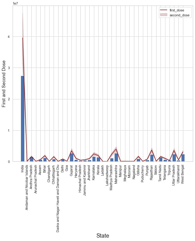
Means the first dose rate is higher than second

Now, checking for which state has highest no. of genderwise vaccination done :-

plt.figure(figsize=(9,8))
sns.set_style('whitegrid', rc={"lines.linewidth": 0.9},)
sns.barplot(vaccination_data['State'],vaccination_data['Male(Individuals Vaccinated)'],color='green',label='Male')
sns.lineplot(vaccination_data['State'],vaccination_data['Female(Individuals Vaccinated)'],color='red',label='Female',palette='muted')
sns.lineplot(vaccination_data['State'],vaccination_data['Transgender(Individuals Vaccinated)'],color='blue',label='Trans',palette='muted')

plt.tight_layout()
plt.xticks(rotation=90)
#plt.legend(['Male'])
plt.ylabel('Vaccinated per (10,000,000)',fontsize=15)
plt.xlabel('State', fontsize=18)

plt.show()

Output:-

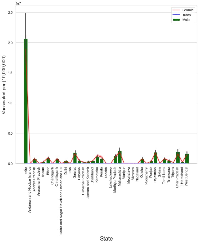
No. of males vaccinated more than females and the TOP states are

1.Maharastra

2.Gujrat

3.Uttar Pradesh

4.Rajasthan

5.West bangal

6.Madhya Pradesh
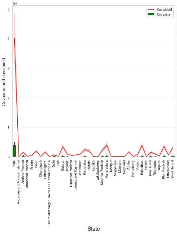
Now,checking for which vaccine is more distribtes:-

plt.figure(figsize=(9,8))
sns.set_style('whitegrid', rc={"lines.linewidth": 0.9},)

sns.lineplot(vaccination_data['State'],vaccination_data['Total CoviShield Administered'],color='red',label='Covishield',palette='muted')
sns.barplot(vaccination_data['State'],vaccination_data['Total Covaxin Administered'],color='green',label='Covaxine')


plt.tight_layout()
plt.xticks(rotation=90)

plt.ylabel('Covaxine and covishield ',fontsize=15)
plt.xlabel('State', fontsize=18)

plt.show()

Output:-

Another Representation is:-

plt.figure(figsize=(9,7))
sns.set_style('whitegrid')
Covaxin = vaccination_data["Total Covaxin Administered"].sum() 
Covishield = vaccination_data["Total CoviShield Administered"].sum() 

plt.pie(x=[Covaxin,Covishield], autopct="%.1f%%" ,labels=['Covaxin','covishield'], pctdistance=0.5);

Output:-

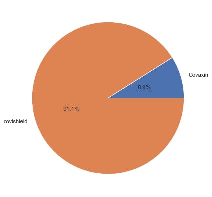
Means covishield is more in production

Now checking which age group is more vaccinated:-

plt.figure(figsize=(9,8))
sns.set_style('whitegrid', rc={"lines.linewidth": 0.9},)
sns.lineplot(vaccination_data['State'],vaccination_data['18-30 years(Age)'],color='green',label='18-30')
sns.lineplot(vaccination_data['State'],vaccination_data['30-45 years(Age)'],color='red',label='30-45',palette='muted')
sns.lineplot(vaccination_data['State'],vaccination_data['45-60

years(Age)'],color='blue',label='45-60',palette='muted')
sns.lineplot(vaccination_data['State'],vaccination_data['60+ years(Age)'],color='maroon',label='60+',palette='muted')
plt.tight_layout()
plt.xticks(rotation=90)
#plt.legend(['Male'])
plt.ylabel('Vaccinated per (10,00000)',fontsize=15)
plt.xlabel('State', fontsize=18)

plt.show()

Output:-

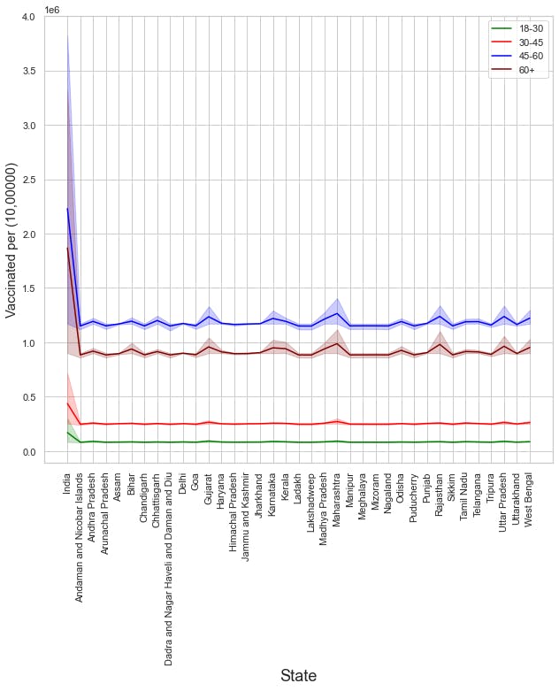
Means 60+ and 45-60 groups are the groups with higher vaccination rate

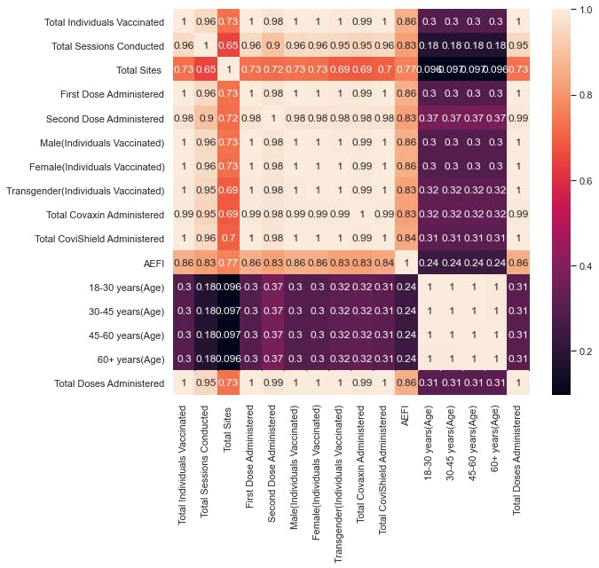
Now, checking for correlation to extract the features:-

cor=vaccination_data.corr()
fet=cor.index
plt.figure(figsize=(9,8))
sns.heatmap(vaccination_data[fet].corr(),annot=True)
plt.show()

Output:-

Labels to include:-

label_vaccination=['Total Individuals Vaccinated','Total Sessions Conducted','AEFI']
X_vacc=vaccination_data[label_vaccination]
Y_vacc=vaccination_data['Total Doses Administered']

Importing and setting up our train and test data:-

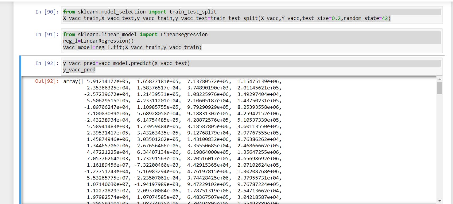
from sklearn.model_selection import train_test_split
X_vacc_train,X_vacc_test,y_vacc_train,y_vacc_test=train_test_split(X_vacc,Y_vacc,test_size=0.2,random_state=42)

from sklearn.linear_model import LinearRegression
reg_l=LinearRegression()
vacc_model=reg_l.fit(X_vacc_train,y_vacc_train)

y_vacc_pred=vacc_model.predict(X_vacc_test)
y_vacc_pred

Output:-

Screenshot (34).png

Checking Accuracy of our model:-

from sklearn.metrics import r2_score

print('Accuracy :',r2_score(y_vacc_test,y_vacc_pred))

Output:- Accuracy : 0.999419968298392

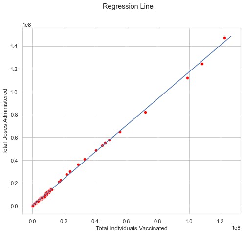
Now, plotting Regression Line:-

y_vaccs=vacc_model.predict(X_vacc_train)
m,b=np.polyfit(X_vacc_train['Total Individuals Vaccinated'],y_vaccs,1)

plt.figure(figsize=(8,7))
sns.set_style('whitegrid')
plt.suptitle('Regression Line')
sns.scatterplot(X_vacc_test['Total Individuals Vaccinated'], y_vacc_test, color = "red")
sns.lineplot(X_vacc_train['Total Individuals Vaccinated'],m*X_vacc_train['Total Individuals Vaccinated']+b)
plt.show()

Output:-

Awesome:), this is the end of this blog about the Analysis of Covid19 in india, but i will come back with another awesome model/project and yes if you want me to do some special project according to your need please write that into the comment section ,i will be pleased to work on that ,till then

Thank You:)

Radhesh's Blog

Radhesh's Blog

COVID 19 Analysis(India)

2020-21

Downloading the dataset:

Importing necessory libraries:-

Now,checking the relationship between deaths , cure and confirm cases in states:

Now, for Recovery Rate:-

Now, checking the Rate of Deaths V/S Rates of Recovery:-

Now, Checking the vaccination:-

Now,checking relationship between total individuas vaccinated and session:-

Now, checking the Difference B/W first dose and second dose:-

Now, checking for which state has highest no. of genderwise vaccination done :-

No. of males vaccinated more than females and the TOP states are

Now,checking for which vaccine is more distribtes:-

Now checking which age group is more vaccinated:-

Now, checking for correlation to extract the features:-

Now, plotting Regression Line:-